Does it matter which model for the extent of Fe oxidation in silicate melt is chosen for calculations?

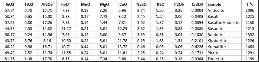
Table 1. Compositions of silicate melts used to assess the impact of Fe oxidation models on the calculations

All calculations used for comparing pseudo-liquidus temperatures and mineral compositions shown on Figures 1 - 5 were done at 1 atm pressure at the QFM buffer of oxygen fugacity. Liquidus temperatures of all compositions but boninite, komatiite and picrite reflect pseudo-liquidus temperature of olivine, and for the latter three compositions they reflect pseudo-liquidus temperatures of spinel (Table 1).

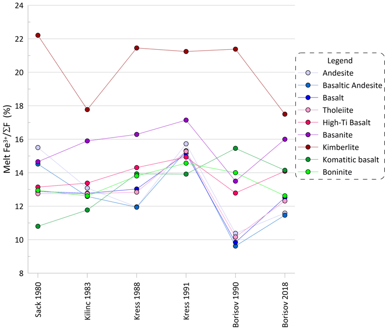
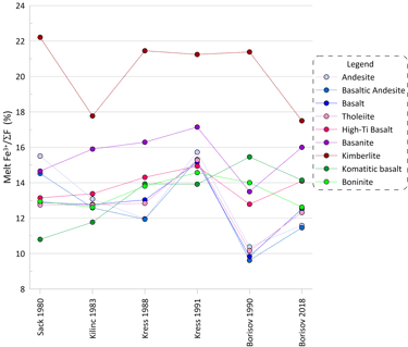
The proportions of ferric Fe as calculated for each of the nine compositions at their liquidus temperatures clearly demonstrate the impact of melt composition on melt oxidation state (Fig. 1). All models predict the highest proportions of ferric Fe in kimberlite and the lowest proportions in basalt, tholeiite, basaltic andesite and komatiitic basalt.

The results also reveal a wide range of the extent of Fe oxidation predicted by different models for a given composition (Fig. 1). Please refer to the original publications for details of formulations of each model that lead to the observed differences (all references are provided in the Petrolog4 manual). The largest impact of the melt composition on the calculated proportions of ferric Fe are displayed by the Sack et al. (1980) and Borisov and Shapkin (1990) models, with both showing variations between ~10% and ~22% of ferric Fe among the 9 compositions. The smallest effects are shown by the Kilinc et al (1983) and Borisov et al (2018) models, with variations between ~ 11% and 18%.

Fe oxidation models determine the proportion of ferric Fe ( Fe3+ / (Fe2+ + Fe3+) ) in the silicate melt during calculations.

Petrolog4 offers a choice of 6 models that were developed between 1980 and 2018. To assess the impact that choosing a specific model may have on the result of calculations, we have selected 9 melt compositions that cover a substantial portion of the compositional spectrum of silicate magmas (Table 1).

Figure 1. Proportions of ferric Fe calculated for the 9 compositions by the six Fe oxidation models.

The observed variations in the proportions of ferric Fe predicted by different models have negligible effect on the pseudo-liquidus temperatures of silicate minerals (olivine is shown as an example in Fig. 2), and thus the set of silicate minerals on the liquidus of the melt is not affected by the choice of the Fe oxidation model.

There is a more pronounced effect, albeit still minor, on the proportions between magnesium and ferrous Fe in ferromagnesian silicate minerals (olivine is shown as an example in Fig. 3). The largest difference of ~ 1 mol% of Mg/(Mg + Fe2+) values is observed between olivine compositions calculated on the liquidus of basalt/tholeiite when using the models of Kress and Carmichael (1991) and Borisov and Shapkin (1990).

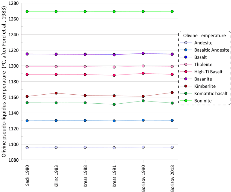
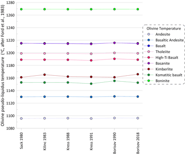
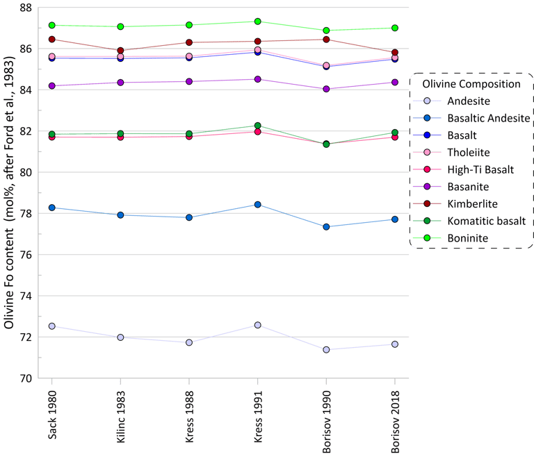
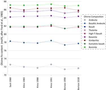
Figure 2. Olivine pseudo-liquidus temperatures calculated for the 9 compositions for each of the six Fe oxidation models.

Figure 3. Olivine forsterite content calculated for the 9 compositions for each of the six Fe oxidation models.

More substantial differences are observed for pseudo-liquidus temperatures and compositions of oxide minerals calculated when using different Fe oxidation models (spinel is shown as an example in Figs 4 and 5). When using the model of Ariskin and Nikolaev (1996), the impact of the Fe oxidation model is most pronounced for melt compositions with low Cr contents.

Note that the impact of the choice of the Fe oxidation model on the calculations depends on the specific formulations of oxide-melt equilibrium models. Some of the models use oxygen fugacity, rather than the proportion of ferric Fe in the melt, to determine the pseudo-liquidus temperature and mineral composition. Such oxide-melt models are not affected by the choice of the Fe oxidation model when calculations are performed using an open system for oxygen (i.e., when oxygen fugacity is controlled by a buffer). Please refer to the original publications for details of formulations of each model (all references are provided in the Petrolog4 manual).

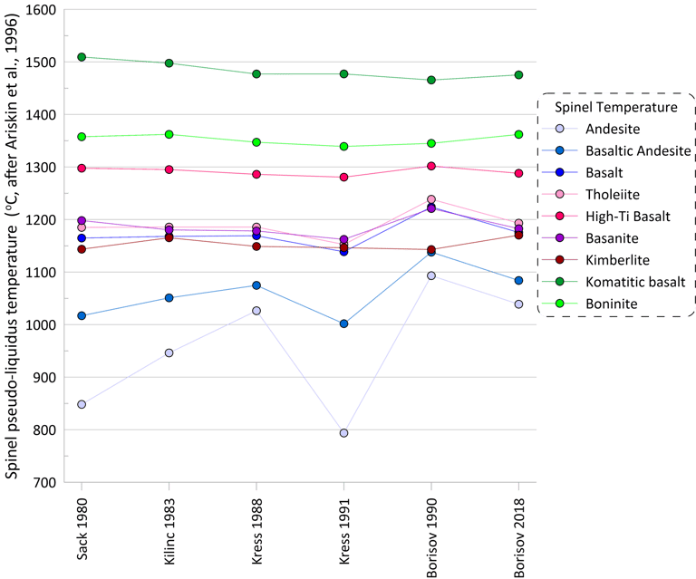
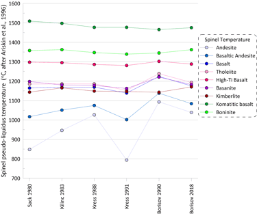
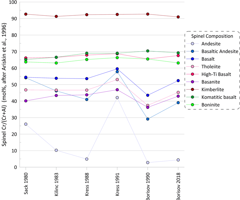
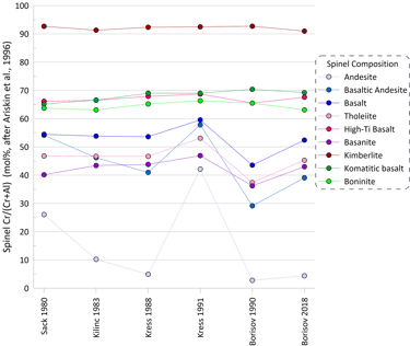
Figure 5. Spinel Cr/(Cr+Al) values (in mol %) calculated for the 9 compositions for each of the six Fe oxidation models.

Figure 4. Spinel pseudo-liquidus temperatures calculated for the 9 compositions for each of the six Fe oxidation models.

To assess the extent to which the choice of Fe oxidation models may affect the calculated fractionation trends (also referred to as liquid lines of descent), we modelled fractional crystallisation of the Basalt composition from Table 1 using two different sets of mineral-melt equilibrium models.

Set I involved models of Bychkov et al. (2023) for olivine, plagioclase, clinopyroxene and orthopyroxene, whereas Set II involved models of Ariskin et al. (1993) for olivine, plagioclase and clinopyroxene and Bolikhovskaya et al (1996) for orthopyroxene.

In both cases, fractionation of spinel was modelled using the model of Ariskin and Nikolaev (1996); fractionation of magnetite using the model of Ariskin and Barmina (1999); fractionation of immiscible sulphide using the model of Kiseeva et al. (2015); and sulphide saturation using the model of Smythe et al. (2017).

Calculations were done at 1 atm pressure for both open and closed systems for oxygen. For the case of an open system, fO2 corresponded to the QFM buffer, and for the closed system the initial proportion of the ferric Fe in the melt was ~ 11.5 at. %.

All calculation were done using the Fe oxidation models of Kress and Carmichael (1991) and Borisov and Shapkin (1990), as these showed the largest difference in the proportions of ferric Fe in basaltic compositions (Fig. 1).

Overall, there are minor changes to the fractionation trends caused by the choice of the Fe oxidation model, with contents of Fe2O3 and FeO in the melt being affected the most (Figs. 6 and 7). The extent of differences caused by the choice of the Fe oxidation model is similar for calculations performed with different sets of mineral-melt equilibrium models (cf. the upper and lower panels on Figs. 6 and 7).

Differences in the initial Fe2O3 and FeO contents in the melt for calculations performed along the QFM buffer (Fig. 6) reflect the higher proportions of ferric Fe predicted by the model of Kress and Carmichael (1991) (Fig. 1). For calculations performed assuming a closed system for oxygen (Fig. 7), observed differences at higher extents of fractionation between calculations done with the two different Fe oxidation models (blue and red lines on Fig. 7) reflect the impact of different fO2 values, as predicted by the two models, on the compositions and timing of appearance of minerals on the liquidus of the fractionating melt.

Impact on the calculated fractionation trends

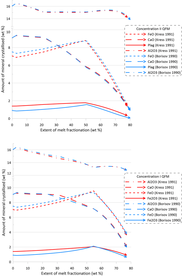
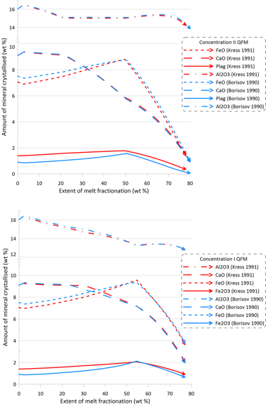
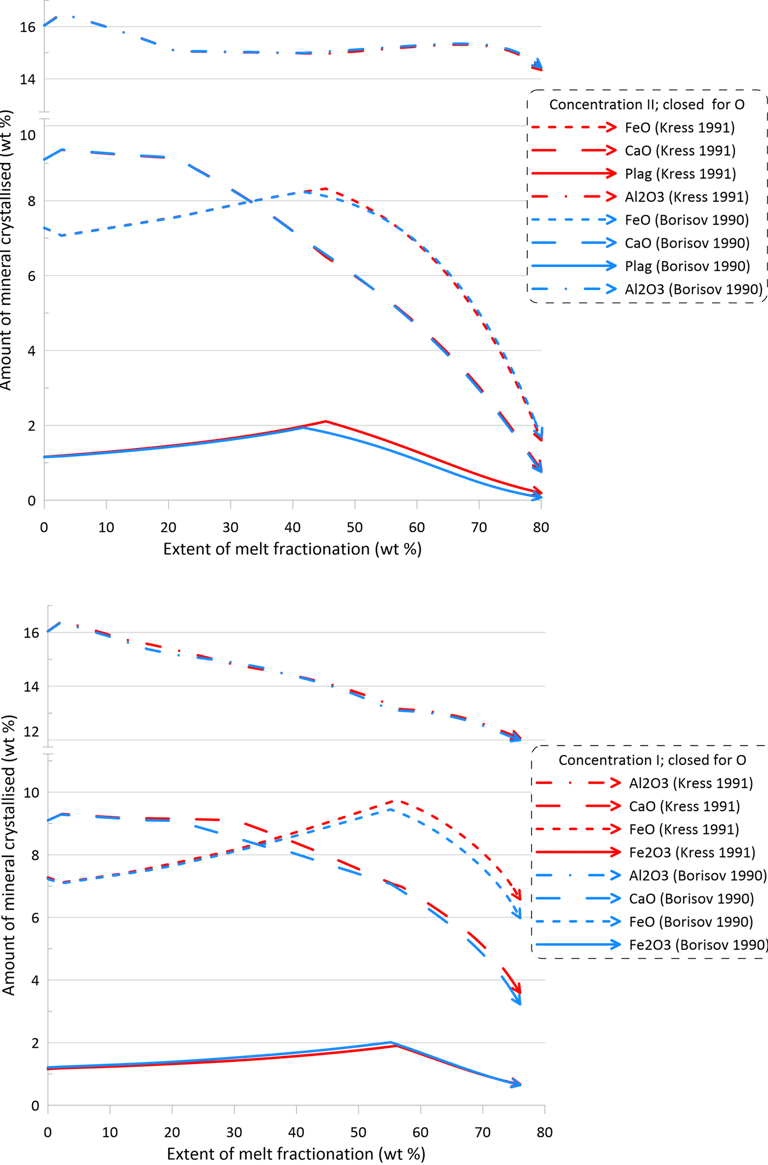
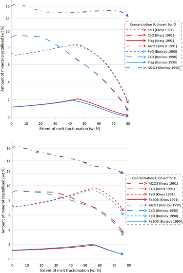
Figure 7. Fractionation trends calculated using the two sets of mineral-melt equilibrium models and two different Fe oxidation models for the case of a system closed for oxygen. See text for details.

Figure 6. Fractionation trends calculated using the two sets of mineral-melt equilibrium models and two different Fe oxidation models for the case of a system open for oxygen. See text for details.

The minor changes in the fractionation trends described above reflect minor effects of the choice of the Fe oxidation model on both the order of crystallisation of the main silicate minerals, and on their proportions during fractionation (Figs. 8 and 9). Note though that there are more pronounced differences in the proportions of olivine and pyroxene when using Set I models (the lower panels of Figs. 8 and 9).

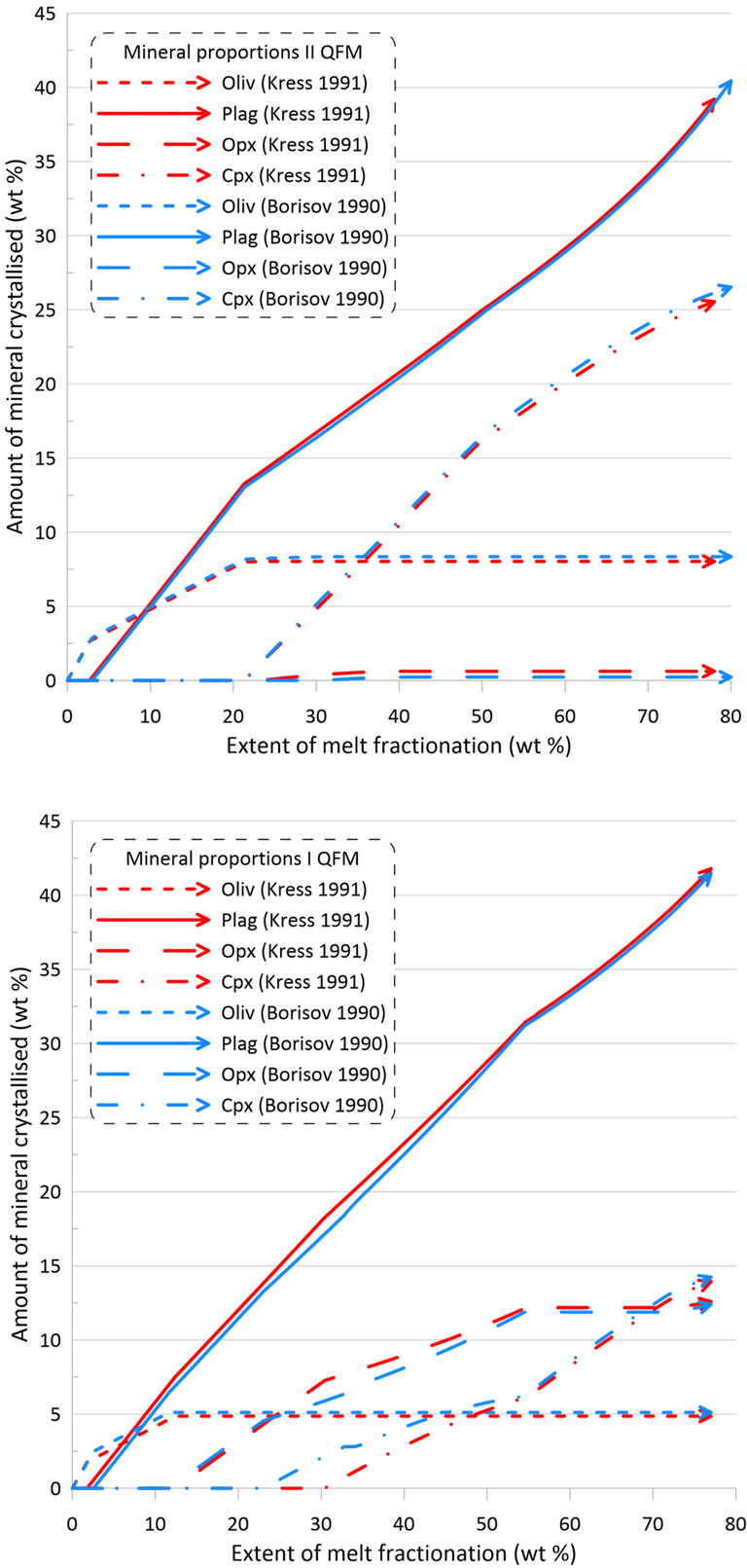
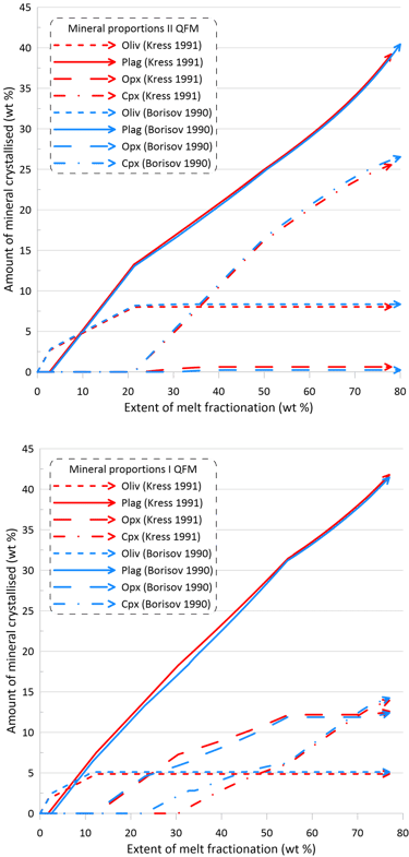
Figure 8. Mineral proportions along the fractionation trends calculated using the two sets of mineral-melt equilibrium models and two different Fe oxidation models for the case of a system open for oxygen. See text for details.

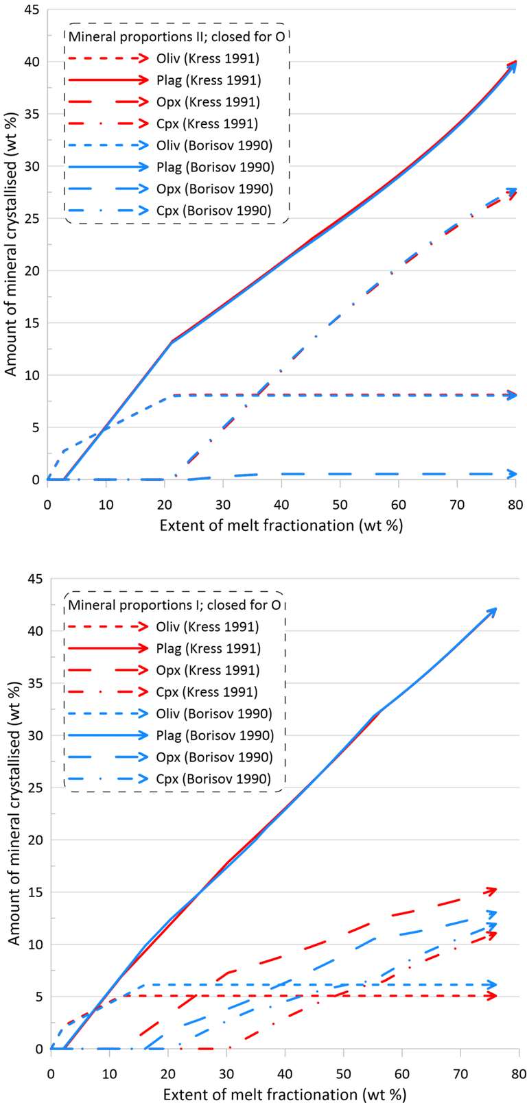
Figure 9. Mineral proportions along the fractionation trends calculated using the two sets of mineral-melt equilibrium models and two different Fe oxidation models for the case of a system closed to oxygen. See text for details.

However, the impact of the choice of the Fe oxidation model is much more significant on oxide minerals and the immiscible sulphide, in terms of both the timing of crystallisation and the proportions of these phases in the crystallising assemblage (Figs. 10 and 11). There is also a more pronounced difference between the sets of mineral-melt equilibrium models with spinel not appearing on the liquidus when using the Kress and Carmichael (1991) model and Set I of mineral-melt equilibrium models. The choice of the Fe oxidation model also causes substantial differences in the timing of spinel crystallisation when doing calculations using Set II (Figs. 10 and 11); in the timing of magnetite crystallisation when doing calculations using Set II and oxidation conditions closed for O (Fig. 11); and in the amount of immiscible sulphide when doing calculations using Set I and oxidation conditions closed for O (Fig. 11).

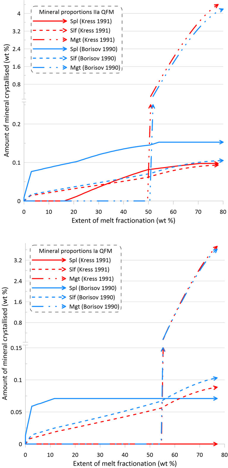
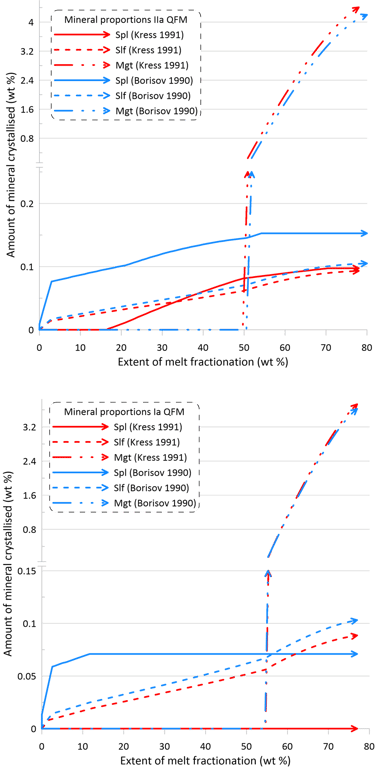
Figure 10. Mineral proportions along the fractionation trends calculated using the two sets of mineral-melt equilibrium models and two different Fe oxidation models for the case of a system open for oxygen. See text for details.

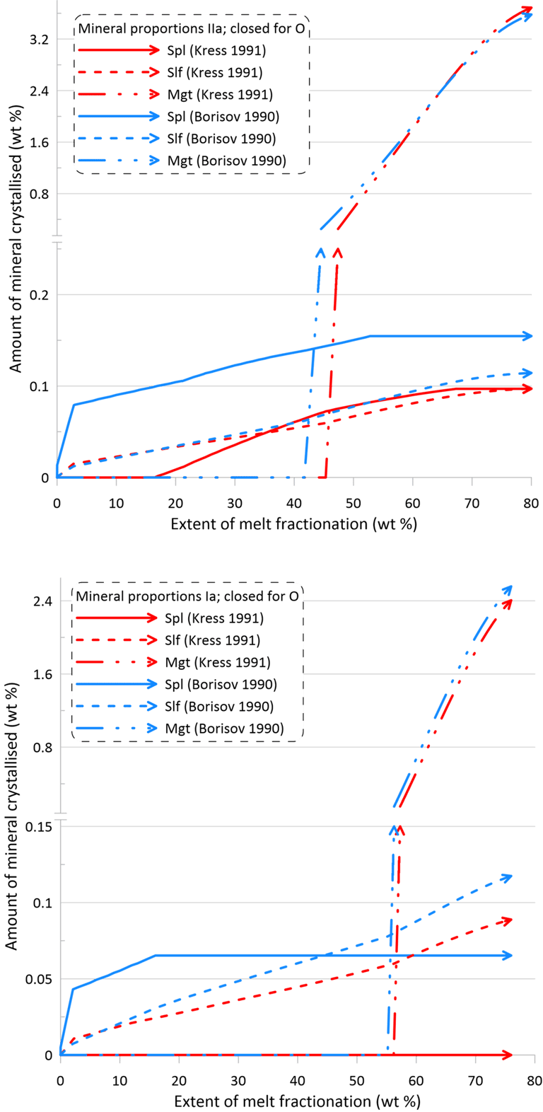
Figure 11. Mineral proportions along the fractionation trends calculated using the two sets of mineral-melt equilibrium models and two different Fe oxidation models for the case of a system closed to oxygen. See text for details.

In summary, the choice of the Fe oxidation model used in calculations may have a significant impact on the crystallisation proportions of oxide minerals and the immiscible sulphide melt.